The data set contains 804 observations (rows) and 18 predictors (columns). The data set contains information about car prices and the variables are described as follows: Price; Mileage; Cylinder; Doors; Cruise; Sound; Leather; Buick; Cadillac; Chevy; Pontiac; Saab; Saturn; convertible; coupe; hatchback; sedan; and wagon.
My first post about statmodels - so be nice! :)
statmodels
Seaborn
Pandas
Python vs. R
Formula API
RDatasets in Python
Patsy in Python
Introduction: Play with GLMs
During my study at HSLU I have learned to use mostly R when it comes to statistic and for some machine learning courses as well. When it comes to work, the most companies I have seen so far, use Python as their main programming language. My previous two employers used Python and R. This article is not going to discuss which language is better, but rather focus on how to use Python and the library statmodels which seems to produce similar outputs as it would in R.
One important and cool thing about the statmodels library is that it has a lot of data sets already included. You can find them here. The data set I use is a R data set from Rdatasets. In particular, the dataset from the package modeldata called car_prices is used.
## Data imports
df = (
    statsmodels.api # imported as sm in following code
    .datasets
    .get_rdataset("car_prices", package='modeldata')
    .data
)
Another important thing about this blog post is the usage of Quarto. Quarto allowed me to write this blog post directly from a Jupyter-Notebook without any fancy and complicated transformations. For more information, please visit the quarto website.
However, let’s start with the analysis. The first thing we do is to import the necessary libraries and the data set.
::: {#code .cell code-fold=‘false’ execution_count=1}
Show the code
## General imports
import warnings
warnings.filterwarnings('ignore')

## Data manipulation imports
import pandas as pd
import numpy as np

## Display imports
from IPython.display import display, Markdown

## statmodels import
import statsmodels.api as sm
import statsmodels.formula.api as smf
import statsmodels.genmod.families.family as fam
from patsy import dmatrices

## Plot imports
import matplotlib.pyplot as plt
plt.rcParams['figure.figsize'] = (5,5/2.5)
import seaborn as sns
sns.set_style('whitegrid')
sns.set_theme()
sns.set_context(
    "paper",
    rc={
        "figsize"       :   plt.rcParams['figure.figsize'],
        'font_scale'    :   1.25,
    }
)


## Data imports
df = (
    sm
    .datasets
    .get_rdataset(
        "car_prices",
        package='modeldata',
    )
    .data
)
:::
Explanatory Data Exploration
The data exploration is a crucial step before fitting a model. It allows to understand the data and to identify potential problems. In this notebook, we will explore very briefly the data, as the focus of this article is to understand and apply statmodels.
First, two approximately continous variables Price and Mileage are investigated by means of graphical analysis. The following bar plots show the distribution of the two variables.
Show the code
height = plt.rcParams['figure.figsize'][0]
aspect = plt.rcParams['figure.figsize'][0]/plt.rcParams['figure.figsize'][1] / 2

g1 = sns.displot(
    data = df,
    x = 'Price',
    kde = True,
    height = height,
    aspect = aspect,
)
plt.title('Distribution of car price')
plt.xlabel('Price')
plt.ylabel('Count of occurance')
plt.show(g1)

g2 = sns.displot(
    data = df,
    x = 'Mileage',
    kde = True,
    height = height,
    aspect = aspect,
)
plt.title('Distribution of Mileage')
plt.xlabel('Mileage')
plt.ylabel('Count of occurance')
plt.show(g2)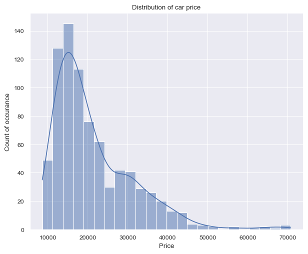
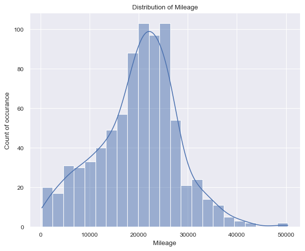
Figure 1 (a) shows on the left a right-skewed distribution with a peak around 15k$ and price values ranging from 8k dollars to 70k dollars. On the other hand, figure 1 (b) shows on the right a more ballanced distribution with a peak around 20k$ and price values ranging from 266 miles up to 50k miles.
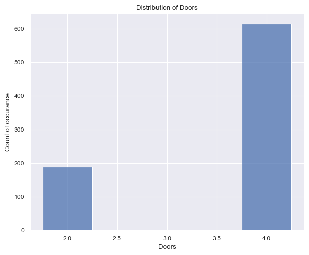
Proceeding to the next two variables, Cylinder and Doors, one can see less possible values, ranging from
Show the code
height = plt.rcParams['figure.figsize'][0]
aspect = plt.rcParams['figure.figsize'][0]/plt.rcParams['figure.figsize'][1] / 2

g = sns.displot(
    data = df,
    x = 'Cylinder',
    discrete = True,
    height = height,
    aspect = aspect,
)
plt.title('Distribution of Cylinder')
plt.xlabel('Cylinder')
plt.ylabel('Count of occurance')
plt.show(g)

# plt.figure()
g = sns.displot(
    data = df,
    x = 'Doors',
    discrete = True,
    shrink = 0.5,
    height = height,
    aspect = aspect,
)
plt.title('Distribution of Doors')
plt.xlabel('Doors')
plt.ylabel('Count of occurance')
plt.show(g)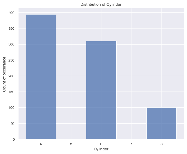
The Figure 2 (a) surprised me quite a bit. I had anticipated the car to feature more than 8 cylinders, given that this dataset pertains to American cars. The cylinder count typically spans from 4 to 8, with the values accurately reflecting this range. It’s worth noting that the number of cylinders is expected to be even.
Again surprisingly, the Figure 2 (b) shows that the number of doors per car. The values are either 2 or 4, with the latter being more common. This is a bit surprising, as I would have expected the number of doors to be higher for American cars (SUV).
Next, we check the distribution of the make of the cars in the dataset. For this analysis, we first pivot the dataframe using pd.melt() and calculate the sum by means of groupby() and sum() method as follows:
Show the code
| variable | value | |
|---|---|---|
| 0 | Buick | 80 |
| 1 | Cadillac | 80 |
| 2 | Chevy | 320 |
| 3 | Pontiac | 150 |
| 4 | Saab | 114 |
After aggregation, the visualization of the data is as follows:
Show the code
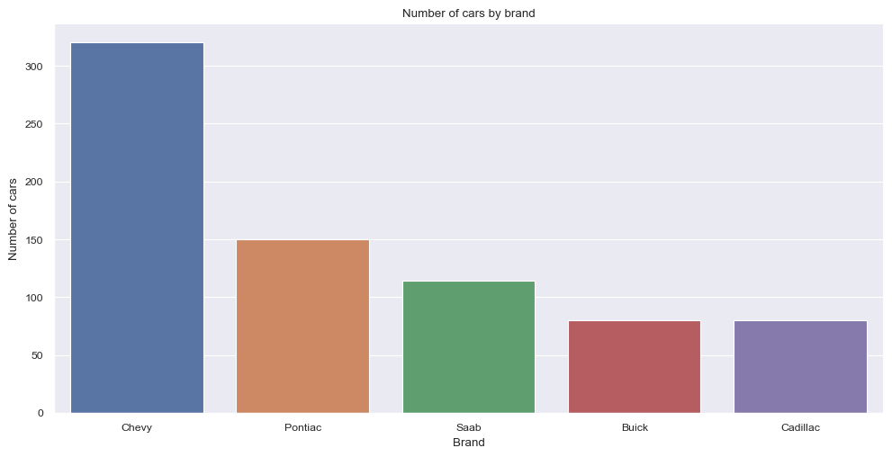
In descending order the most present make is: Chevy followed by Pontiac, Saab, Buick and Cadilac.
At this point it should be mentioned, that the data set is not balanced and the distribution of the features is not uniform across the different makes and car features. In a normal project this would be a point to consider and to take care of. However, for the purpose of this project, this is not necessary.
Modeling
Modeling with statsmodels becomes straightforward once the formula API and provided documentation are well understood. I encountered a minor challenge in grasping the formula API, but once I comprehended it, the usage turned out to be quite intuitive.
Let’s delve into an understanding of the formula API (statsmodels.formula.api). This feature enables us to employ R-style formulas for specifying models. To illustrate, when fitting a linear model, the following formula suffices:
The formula API leverages the patsy package (Patsy Package). It’s worth noting that the formula API’s potency extends to intricate models. Additionally, it’s important to mention that the formula API automatically incorporates an intercept into the formula if one isn’t explicitly specified. For cases where the intercept is undesired, a -1 can be used within the formula.
With the glm class, a vast array of models becomes accessible importing as follows:
The fam import is necessary for specifying the family of the model. The families available are:
| Name | Description |
|---|---|
| Family(link, variance[, check_link]) | The parent class for one-parameter exponential families. |
| Binomial([link, check_link]) | Binomial exponential family distribution. |
| Gamma([link, check_link]) | Gamma exponential family distribution. |
| Gaussian([link, check_link]) | Gaussian exponential family distribution. |
| InverseGaussian([link, check_link]) | InverseGaussian exponential family. |
| NegativeBinomial([link, alpha, check_link]) | Negative Binomial exponential family (corresponds to NB2). |
| Poisson([link, check_link]) | Poisson exponential family. |
| Tweedie([link, var_power, eql, check_link]) | Tweedie family. |
Fitting the model and analyzing the results are the same as one would using R. First define the model, then fit it, then analyze the results. The details of the fit can be accessed using the summary method.
                 Generalized Linear Model Regression Results
==============================================================================
Dep. Variable:                  Price   No. Observations:                  804
Model:                            GLM   Df Residuals:                      789
Model Family:                Gaussian   Df Model:                           14
Link Function:               Identity   Scale:                      8.4460e+06
Method:                          IRLS   Log-Likelihood:                -7544.8
Date:                Sun, 03 Sep 2023   Deviance:                   6.6639e+09
Time:                        21:02:49   Pearson chi2:                 6.66e+09
No. Iterations:                     3   Pseudo R-squ. (CS):              1.000
Covariance Type:            nonrobust
===============================================================================
                  coef    std err          z      P>|z|      [0.025      0.975]
-------------------------------------------------------------------------------
Mileage        -0.1842      0.013    -14.664      0.000      -0.209      -0.160
Cylinder     3659.4543    113.345     32.286      0.000    3437.303    3881.606
Doors        1654.6326    174.525      9.481      0.000    1312.570    1996.695
Cruise        340.8695    295.962      1.152      0.249    -239.205     920.944
Sound         440.9169    234.484      1.880      0.060     -18.664     900.497
Leather       790.8220    249.745      3.167      0.002     301.331    1280.313
Buick       -1911.3752    336.292     -5.684      0.000   -2570.495   -1252.256
Cadillac      1.05e+04    409.274     25.663      0.000    9701.132    1.13e+04
Chevy       -3408.2863    213.274    -15.981      0.000   -3826.295   -2990.278
Pontiac     -4258.9628    256.358    -16.613      0.000   -4761.416   -3756.509
Saab         9419.1227    331.211     28.438      0.000    8769.960    1.01e+04
Saturn      -2859.0803    358.709     -7.970      0.000   -3562.137   -2156.023
convertible  1.258e+04    525.984     23.922      0.000    1.16e+04    1.36e+04
coupe        1559.7620    395.946      3.939      0.000     783.723    2335.801
hatchback   -4977.3196    339.046    -14.680      0.000   -5641.837   -4312.803
sedan       -3064.7176    215.007    -14.254      0.000   -3486.123   -2643.312
wagon        1384.6400    364.920      3.794      0.000     669.410    2099.870
===============================================================================
After fitting a GLM using the glm class in statsmodels, you can obtain a summary of the model’s results using the .summary() method on the fitted model object. Here’s a general overview of the information typically included in the summary output:
- Model Information:
- The name of the model.
- The method used for estimation (e.g., maximum likelihood).
- The distribution family (e.g., Gaussian, binomial, Poisson).
- The link function used in the model (e.g., logit, identity, etc.).
- The number of observations used in the model.
- Model Fit Statistics:
- Log-likelihood value.
- AIC (Akaike Information Criterion) and/or BIC (Bayesian Information Criterion).
- Deviance and Pearson chi-square statistics.
- Dispersion parameter (if applicable).
- Coefficients:
- Estimated coefficients for each predictor variable.
- Standard errors of the coefficients.
- z-scores and p-values for testing the significance of the coefficients.
- Confidence Intervals:
- Confidence intervals for each coefficient, often at a default level like 95%.
- Hypothesis Testing:
- Hypothesis tests for the coefficients, typically with null hypothesis being that the coefficient is zero.
- Goodness of Fit:
- Likelihood-ratio test for overall model fit.
- Tests for assessing the contribution of individual predictors to the model.
- Diagnostic Information:
- Information about model assumptions and diagnostics, depending on the type of GLM and the method used.
- Residuals:
- Information about residuals, which can include measures like deviance residuals, Pearson residuals, etc.
Refer to the official documentation for the most accurate and up-to-date information about the summary output for your specific use case.
Conclusion
Statsmodels is a powerful Python library for statistical modeling and hypothesis testing, making it an excellent transition for R users or Python users who like R to solve certain problems. It offers a familiar syntax and functionality for regression, ANOVA, and more. Its integration with Python’s data analysis ecosystem, like pandas, allows seamless data manipulation. With support for various statistical methods and a comprehensive summary output, Statsmodels facilitates effortless migration from R, enabling R users to harness its capabilities in a Python environment.